Bayes Part 3

Introduction

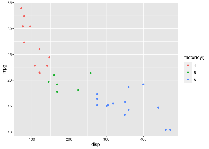
In this post, I’ll work through the mtcars example again but this time using the rstan package. Recall that I’m interested in a model with response mpg and predictor disp.

Setup Environment

First some basic R environment setup.

rm(list=ls())

library(tidyverse)
library(bayesplot)
library(shinystan)
library(rstan)
library(gridExtra)

knitr::opts_chunk$set(out.width = "50%")
knitr::opts_chunk$set(fig.align = "center")
knitr::opts_chunk$set(message=FALSE)
knitr::opts_chunk$set(warning=FALSE)

options("scipen" = 1, "digits" = 4)

set.seed(123)

Setting the the following option saves a compiled version of the model to hard disk, so it only needs to be recompiled if the model is changed.

rstan_options(auto_write = TRUE)
options(mc.cores = parallel::detectCores()-1)

library(datasets)
data(mtcars)
#head(mtcars)

mtcars %>%
  ggplot(aes(x=disp, y=mpg)) +
  geom_point(aes(color=factor(cyl))) 

Linear Model

Again I’ll start with a linear model even though it clearly isn’t going to be a great fit to the data. Like the rethinking package, rstan doesn’t have default priors, so I need to explicitly choose them:

Defining the model in rstan is a bit different since the syntax is more akin to C/C++. For a simple linear model there are three sections to the model definition:

1. data - This is where the data structures for the known/observed portions of the model (e.g., the number of observations, the number and type of predictors) are defined.

2. parameters - This is where the data structures for the parameters to be estimated are defined. For example, the coefficients of the simple linear model belong in this section.

3. model - This is where the model (including priors) is defined using the data structures from the previous sections.

# Define model

mdl_code <- '
  data{
    int<lower=1> N;
    vector[N] mpg;
    vector[N] disp;
  }
  parameters{
    real a;
    real<lower=-0.1, upper=0.0> b;
    real<lower=0.0> sigma;
  }
  model{
    // Likelihood
    mpg ~ normal(a + b * disp, sigma);
    // Priors
    a ~ normal(25, 10);
    b ~ uniform(-0.1, 0.0);
    sigma ~ exponential(0.2);
  }
'

A few comments about the model definition.

1. For those only familiar with R, it may seem like a lot of extra “stuff” is going on in the code and parameters sections. This is because under the hood rstan and stan use C++ which is statically typed, unlike R which is dynamically typed. What that means is you must define the type of any variable before you use it.

2. The lower= and upper= statements define bounds for a variable. The data is checked against the bounds which can detect errors pre-compilation. Generally, bounds are a good idea but aren’t required. Except for…

3. A narrow interval prior, such as for b in the above model, does require both upper and lower bounds be specified. This blog post explains why. And it also explains why narrow interval priors are not a good idea! This had never come up in any of my courses. For the sake of consistency, I’ll leave the model as is so it’s easy to compare against what I did previously with rstanarm and rethinking, but lesson learned for the future.

Next, populate the data structures from the data section and save in a list.

mdl_data <- list(N = nrow(mtcars),
                 mpg = mtcars$mpg,
                 disp = mtcars$disp)

And this is the call to fit the model.

# Fit model
mdl1 <- stan(model_code=mdl_code, data=mdl_data, model_name="mdl")

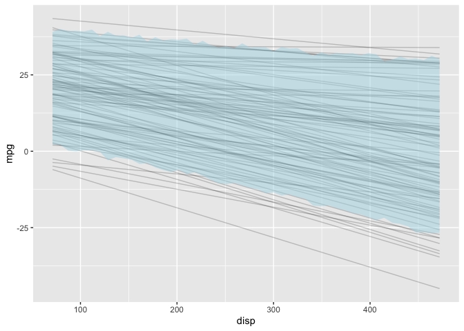
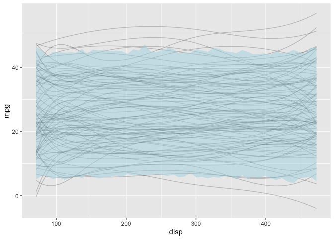
Prior Predictive Distribution

First, I’ll examine the prior predictive distribution to see if the default priors seem reasonable. This model is simple enough that I could manually construct the prior predictive distribution (see example here). But I can also have stan generate the prior predictive distribution which will be useful for more complex models. To do this, I create another model with just the data and generated quantities section. The generated quantities section mirrors the model section except it is now drawing samples from the priors without conditioning on the observed data. Also, in the stan call I need to set the sampling algorithm for fixed parameters.

# Plot prior predictive distribution
mdl_prior <- '
  data{
    int<lower=1> N;
    vector[N] disp;
  }
generated quantities{
  real a_sim = normal_rng(25, 10);
  real b_sim = uniform_rng(-0.1, 0.0);
  real sigma_sim = exponential_rng(0.2);
  real mpg_sim[N] = normal_rng(a_sim + b_sim * disp, sigma_sim);
}
'

N<- 50
D <- seq(min(mtcars$disp), max(mtcars$disp), length.out = N)
mdl_data_prior <- list(N = N, disp=D)

mdl_prior <- stan(model_code=mdl_prior, data=mdl_data_prior, model_name="mdl_prior",
             chains=1, algorithm="Fixed_param")

draws <- as.data.frame(mdl_prior) %>%
  head(100)

# Expected value prior predictive distribution
exp_mpg_sim <- apply(draws, 1, function(x) x["a_sim"] + x["b_sim"]*D) %>%
  as.data.frame() %>%
  mutate(disp = D) %>%
  pivot_longer(-c("disp"), names_to="iter", values_to="mpg") 

# 89% interval prior predictive distribution
mpg_sim <- as.data.frame(mdl_prior) %>% select(starts_with("mpg")) %>%
  apply(2, function(x) quantile(x, probs=c(0.055, 0.945))) %>%
  t() %>%
  as.data.frame() %>%
  mutate(disp = D)

ggplot() +
  geom_line(data=exp_mpg_sim, mapping=aes(x=disp, y=mpg, group=iter), alpha=0.2) +
  geom_ribbon(data=mpg_sim, mapping=aes(x=disp, ymin=`5.5%`, ymax=`94.5%`), 
              alpha=0.5, fill="lightblue")

Diagnostic Plots

Since the priors looks reasonable, the next step is to examine the diagnostic plots for the fitted model.

mcmc_trace(mdl1, pars=c("a", "b", "sigma"))

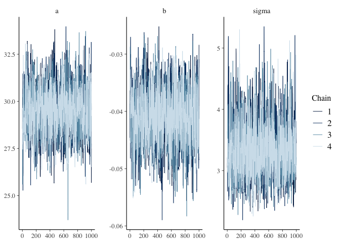
Recall that there are three things I am looking for in the trace plot of each chain–good mixing, stationarity and convergence. The trace plots above look good in all three respects.

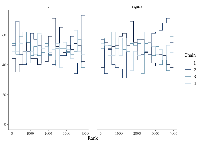
Trace Rank Plot

mcmc_rank_overlay(mdl1, pars=c("b", "sigma"))

Effective Sample Size

print(mdl1)

## Inference for Stan model: mdl.
## 4 chains, each with iter=2000; warmup=1000; thin=1; 
## post-warmup draws per chain=1000, total post-warmup draws=4000.
## 
##         mean se_mean   sd   2.5%    25%    50%    75%  97.5% n_eff Rhat
## a      29.56    0.03 1.25  27.11  28.74  29.58  30.38  32.05  1549    1
## b      -0.04    0.00 0.00  -0.05  -0.04  -0.04  -0.04  -0.03  1448    1
## sigma   3.34    0.01 0.45   2.58   3.02   3.30   3.61   4.37  1624    1
## lp__  -57.59    0.04 1.27 -60.76 -58.20 -57.28 -56.65 -56.12  1158    1
## 
## Samples were drawn using NUTS(diag_e) at Sat Nov 28 13:58:38 2020.
## For each parameter, n_eff is a crude measure of effective sample size,
## and Rhat is the potential scale reduction factor on split chains (at 
## convergence, Rhat=1).

Posterior Distribution

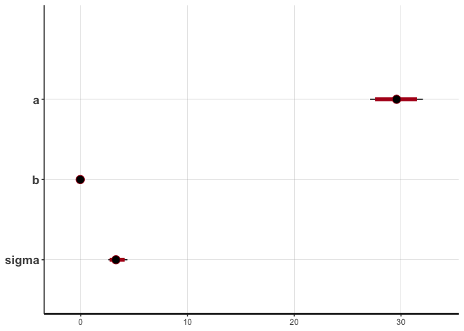
The print function above displays information about the posterior distributions in addition to n_eff. Alternatively, the plot function provides a graphical display of the posterior distributions.

plot(mdl1, ci_level=0.89)

Posterior Predictive Distribution

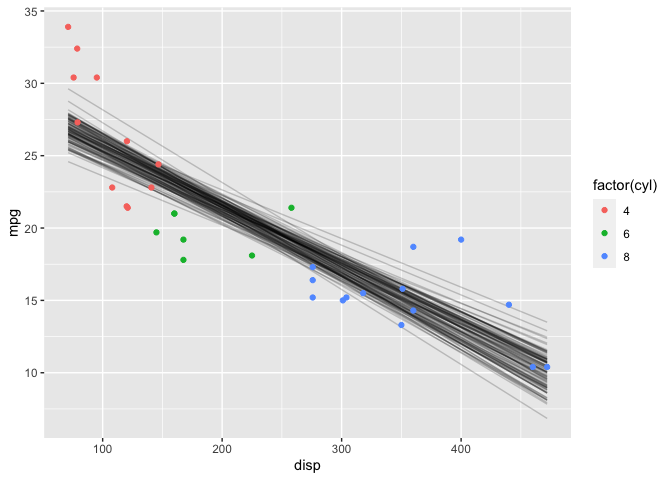
Finally, I’ll check the posterior predictive distribution (ppd). Using the posterior samples, I can plot individual lines for the expected value of the ppd.

N<- 50
D <- seq(min(mtcars$disp), max(mtcars$disp), length.out = N)

draws <- as.data.frame(mdl1) %>%
  head(100)

# Expected value posterior predictive distribution
post_pred <- apply(draws, 1, function(x) x["a"] + x["b"]*D) %>%
  as.data.frame() %>%
  mutate(disp = D) %>%
  pivot_longer(-c("disp"), names_to="iter", values_to="mpg") 

ggplot() +
  geom_line(data=post_pred, mapping=aes(x=disp, y=mpg, group=iter), alpha=0.2) +
  geom_point(data=mtcars, mapping=aes(x=disp, y=mpg, color=factor(cyl)))

However, the expected value of the ppd doesn’t include (\sigma). It’s possible to have stan automatically generate samples from the posterior predictive distribution itself by adding a generated quantities section to the model (similar to what I did for the prior predictive distribution).

# Define model

mdl_code_ppd <- '
  data{
    int<lower=1> N;
    vector[N] mpg;
    vector[N] disp;
  }
  parameters{
    real a;
    real<lower=-0.1, upper=0.0> b;
    real<lower=0.0> sigma;
  }
  transformed parameters{
    vector[N] Y_hat = a + b * disp;
  }
  model{
    // Likelihood
    mpg ~ normal(Y_hat, sigma);
    // Priors
    a ~ normal(25, 10);
    b ~ uniform(-0.1, 0.0);
    sigma ~ exponential(0.2);
  }
  generated quantities{
    // Posterior Predictive
    real mpg_ppd[N] = normal_rng(Y_hat, sigma);
  }
'

# Fit model
mdl1_ppd <- stan(model_code=mdl_code_ppd, data=mdl_data)

draws <- as.data.frame(mdl1_ppd) %>%
  select(starts_with("mpg")) %>%
  apply(2, fivenum) %>%  
  t() %>%
  as.data.frame()

dat <- mtcars %>%
  select(c("mpg", "disp")) %>%
  rownames_to_column(var="car") 

cbind(dat, draws) %>%
  ggplot(aes(x=fct_reorder(car, disp))) +
  geom_boxplot(mapping=aes(ymin=V1, lower=V2, middle=V3, upper=V4, ymax=V5),
               stat="identity",
               outlier.shape = NA) +
  geom_point(mapping=aes(y=mpg), color="red") +
  theme(axis.text.x = element_text(angle = 90))

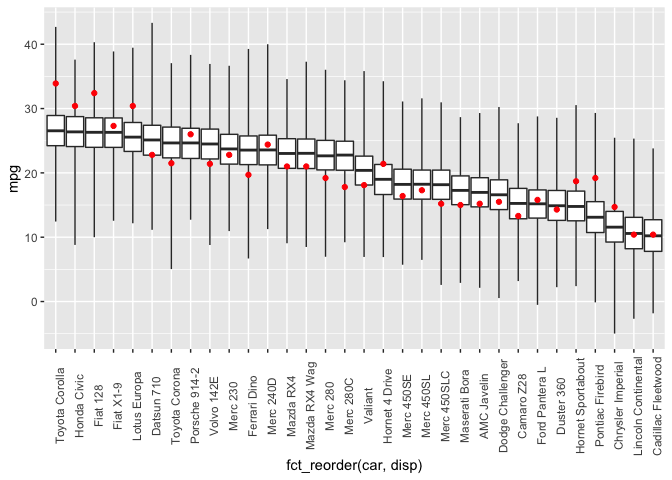
As expected, the linear model isn’t a great fit to the data, but the results are consistent with what I got previously using both rstanarm and rethinking.

Generalized Additive Model

First, I’ll define the splines just as I did when using the rethinking package.

library(splines)

num_knots <- 4  # number of interior knots
knot_list <- quantile(mtcars$disp, probs=seq(0,1,length.out = num_knots))
B <- bs(mtcars$disp, knots=knot_list[-c(1,num_knots)], intercept=TRUE)

df1 <- cbind(disp=mtcars$disp, B) %>%
  as.data.frame() %>%
  pivot_longer(-disp, names_to="spline", values_to="val")

# Plot at smaller intervals so curves are smooth
N<- 50
D <- seq(min(mtcars$disp), max(mtcars$disp), length.out = N)
B_plot <- bs(D, 
             knots=knot_list[-c(1,num_knots)], 
             intercept=TRUE)

df2 <- cbind(disp=D, B_plot) %>%
  as.data.frame() %>%
  pivot_longer(-disp, names_to="spline", values_to="val")

ggplot(mapping=aes(x=disp, y=val, color=spline)) +
  geom_point(data=df1) +
  geom_line(data=df2, linetype="dashed")

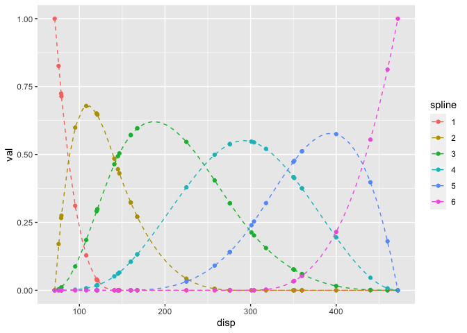
Note: the dashed lines are the splines and the points are the values of the spline at the specific values of mtcars$disp; the points are inputs into the stan model.

Prior Predictive Distribution

# Define model

mdl2 <- '
  data{
    int<lower=1> N;
    int<lower=1> num_basis;
    //vector[N] mpg;
    //vector[N] disp;
    matrix[N, num_basis] B;
  }
  generated quantities{
    real a_sim = normal_rng(25, 10);
    real sigma_sim = exponential_rng(0.2);
    real mpg_sim[N];
    vector[num_basis] w_sim;
    for (i in 1:num_basis)
      w_sim[i] = normal_rng(0,5);
    mpg_sim = normal_rng(a_sim + B * w_sim, sigma_sim);
}
'

mdl_data_prior <- list(N=N, 
                 num_basis=ncol(B_plot),
                 B=B_plot)

mdl_gam_prior <- stan(model_code=mdl2, 
                      data=mdl_data_prior,
             chains=1, algorithm="Fixed_param")

draws <- as.data.frame(mdl_gam_prior) %>%
  head(100)

# Expected value prior predictive distribution
exp_mpg_sim <- apply(draws, 1, function(x) {
  x["a_sim"] + B_plot %*% x[grepl("w", names(x))]
}) %>%
  as.data.frame() %>%
  mutate(disp = D) %>%
  pivot_longer(-c("disp"), names_to="iter", values_to="mpg") 

# 89% interval prior predictive distribution
mpg_sim <- as.data.frame(mdl_gam_prior) %>% select(starts_with("mpg")) %>%
  apply(2, function(x) quantile(x, probs=c(0.055, 0.945))) %>%
  t() %>%
  as.data.frame() %>%
  mutate(disp = D)

ggplot() +
  geom_line(data=exp_mpg_sim, mapping=aes(x=disp, y=mpg, group=iter), alpha=0.2) +
  geom_ribbon(data=mpg_sim, mapping=aes(x=disp, ymin=`5.5%`, ymax=`94.5%`), 
              alpha=0.5, fill="lightblue")

Posterior

# Define model

mdl_code <- '
  data{
    int<lower=1> N;
    int<lower=1> num_basis;
    vector[N] mpg;
    vector[N] disp;
    matrix[N, num_basis] B;
  }
  parameters{
    real a;
    real<lower=0.0> sigma;
    vector[num_basis] w;
  }
  transformed parameters{
    vector[N] Y_hat = a + B*w;
  }
  model{
    // Likelihood
    mpg ~ normal(Y_hat, sigma);
    // Priors
    a ~ normal(25, 10);
    sigma ~ exponential(0.2);
    w ~ normal(0, 5);
  }
  generated quantities{
    // Posterior Predictive
    real mpg_ppd[N] = normal_rng(Y_hat, sigma);
  }
'

mdl_data <- list(N=nrow(mtcars),
                 num_basis=ncol(B),
                 B=B,
                 mpg = mtcars$mpg,
                 disp = mtcars$disp)

# Fit model
mdl1_gam <- stan(model_code=mdl_code, data=mdl_data)

print(mdl1_gam, pars=c("a", "sigma", "w"))

## Inference for Stan model: 7ae6bef6fd6e1ad16f99577e64710ecd.
## 4 chains, each with iter=2000; warmup=1000; thin=1; 
## post-warmup draws per chain=1000, total post-warmup draws=4000.
## 
##        mean se_mean   sd   2.5%    25%   50%   75% 97.5% n_eff Rhat
## a     20.22    0.07 2.08  16.11  18.84 20.23 21.58 24.35  1009 1.01
## sigma  2.31    0.01 0.34   1.75   2.07  2.28  2.52  3.06  2469 1.00
## w[1]  11.84    0.07 2.43   7.10  10.29 11.84 13.47 16.42  1229 1.01
## w[2]   4.32    0.07 2.71  -1.04   2.47  4.30  6.16  9.67  1515 1.00
## w[3]  -0.60    0.08 2.96  -6.39  -2.60 -0.56  1.39  5.12  1436 1.00
## w[4]  -5.65    0.08 3.09 -11.51  -7.75 -5.71 -3.57  0.53  1538 1.00
## w[5]  -2.41    0.08 3.05  -8.50  -4.46 -2.35 -0.41  3.59  1637 1.00
## w[6]  -8.81    0.07 2.54 -13.58 -10.53 -8.89 -7.08 -3.73  1244 1.00
## 
## Samples were drawn using NUTS(diag_e) at Sat Nov 28 14:00:52 2020.
## For each parameter, n_eff is a crude measure of effective sample size,
## and Rhat is the potential scale reduction factor on split chains (at 
## convergence, Rhat=1).

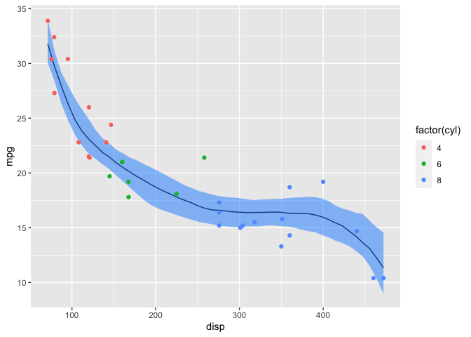
Posterior Predictive Distribution

Finally, I’ll examine the posterior predictive distribution (ppd). One method is to manually calculate the expected value of the ppd (i.e., does not incorporate (\sigma)) and plot the 89% credible interval.

draws <- as.data.frame(mdl1_gam) %>%
  head(100)

# Method 1: Manually calculate credible interval for expected value of ppd
post_pred <- apply(draws, 1, function(x) {
  x["a"] + B_plot %*% x[grepl("w", names(x))]
}) %>%
  apply(1, function(x) quantile(x, probs=c(0.055, 0.5, 0.945))) %>%
  t() %>%
  as.data.frame() %>%
  mutate(disp = D) 

ggplot(post_pred) +
  geom_line(mapping=aes(x=disp, y=`50%`)) +
  geom_ribbon(mapping=aes(x=disp, ymin=`5.5%`, ymax=`94.5%`), 
              alpha=0.5, fill="dodgerblue") +
  geom_point(data=mtcars, mapping=aes(x=disp, y=mpg, color=factor(cyl))) +
  labs(y="mpg")

Alternatively, I can plot the 89% credible intervals for the ppd (which includes (\sigma)) and expected value of the ppd from the mpg_ppd and Y_hat draws that were generated automatically by stan.

# Method 2: Calculate 89% interval for expected value of posterior predictive from Y_hat
Epost_pred <- draws %>% select(starts_with("Y_hat")) %>%
  apply(2, function(x) quantile(x, probs=c(0.055, 0.5, 0.945))) %>%
  t() %>%
  as.data.frame() %>%
  mutate(disp = mtcars$disp)

# Method 3: Use posterior predictive from generated quantities

post_pred <- draws %>% select(starts_with("mpg")) %>%
  apply(2, function(x) quantile(x, probs=c(0.055, 0.5, 0.945))) %>%
  t() %>%
  as.data.frame() %>%
  mutate(disp = mtcars$disp)

ggplot(Epost_pred) +
  geom_line(mapping=aes(x=disp, y=`50%`)) +
  geom_ribbon(data=post_pred,
              mapping=aes(x=disp, ymin=`5.5%`, ymax=`94.5%`), 
              alpha=0.5, fill="lightblue") +
    geom_ribbon(mapping=aes(x=disp, ymin=`5.5%`, ymax=`94.5%`), 
              alpha=0.5, fill="dodgerblue") +
  geom_point(data=mtcars, mapping=aes(x=disp, y=mpg, color=factor(cyl))) +
  labs(y="mpg")

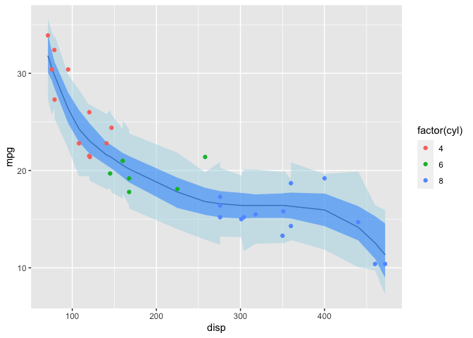
Note that the darker credible interval above is equivalent to interval I previously calculated manually. The reason the intervals in this plot don’t look as smooth is because I specified the model such that Y_hat and mpg_ppd draws are only at the specific values of mtcars$disp.

Alternative model

One challenge with splines is choosing the number of knots. For the previous model, I tried several values for num_knots until settling on 4. However, there is a stan case study for splines that uses a novel prior which addresses this issue. The details are here.

library(splines)

num_knots <- 20  # number of interior knots
knot_list <- quantile(mtcars$disp, probs=seq(0,1,length.out = num_knots))
B <- bs(mtcars$disp, knots=knot_list[-c(1,num_knots)], intercept=TRUE)

# Define model with smoothing prior
mdl_smooth_code <- '
  data{
    int<lower=1> N;
    int<lower=1> num_basis;
    vector[N] mpg;
    vector[N] disp;
    matrix[N, num_basis] B;
  }
  parameters{
    real a;
    real<lower=0.0> sigma;
    vector[num_basis] w_raw;
    real<lower=0.0> tau;
  }
  transformed parameters{
    vector[num_basis] w;
    vector[N] Y_hat;
    w[1] = w_raw[1];
    for (i in 2:num_basis)
      w[i] = w[i-1] + w_raw[i]*tau;
    Y_hat = a + B*w;
  }
  model{
    // Likelihood
    mpg ~ normal(Y_hat, sigma);
    // Priors
    a ~ normal(25, 10);
    sigma ~ exponential(0.2);
    w_raw ~ normal(0, 1);
    tau ~ normal(0,1);
  }
  generated quantities{
    real mpg_ppd[N] = normal_rng(a + B*w, sigma);
  }
'

mdl_data <- list(N=nrow(mtcars), 
                 num_basis=ncol(B),
                 B=B,
                 mpg = mtcars$mpg,
                 disp = mtcars$disp)

# Fit model with smoothing prior
mdl2_gam_smooth <- stan(model_code=mdl_smooth_code, data=mdl_data,
                 control=list(adapt_delta=0.99))

# Fit model without smoothing prior
mdl2_gam <- stan(model_code = mdl_code, data=mdl_data,
                 control=list(adapt_delta=0.99))

draws <- as.data.frame(mdl2_gam) %>% head(100)

Epost_pred <- draws %>% select(starts_with("Y_hat")) %>%
  apply(2, function(x) quantile(x, probs=c(0.055, 0.5, 0.945))) %>%
  t() %>%
  as.data.frame() %>%
  mutate(disp = mtcars$disp)

draws_smooth <- as.data.frame(mdl2_gam_smooth) %>% head(100)

Epost_pred_smooth <- draws_smooth %>% select(starts_with("Y_hat")) %>%
  apply(2, function(x) quantile(x, probs=c(0.055, 0.5, 0.945))) %>%
  t() %>%
  as.data.frame() %>%
  mutate(disp = mtcars$disp)

rbind(Epost_pred %>% select(c("disp", `50%`)) %>% mutate(type="without smoothing prior"),
      Epost_pred_smooth %>% select(c("disp", `50%`)) %>% mutate(type="with smoothing prior")) %>%
  ggplot() +
  geom_line( mapping=aes(x=disp, y=`50%`, linetype=type) ) +
  geom_point(data=mtcars, mapping=aes(x=disp, y=mpg, color=factor(cyl))) +
  labs(y="mpg")

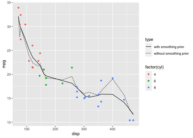
The plot above shows that even with a large number of knots (in this case 20), the model with the smoothing prior significantly reduces over-fitting when compared to the model without the smoothing prior. The model without the smoothing prior gives similar results as to the fit I did with the rethinking package here.